import numpy as np
import matplotlib.pyplot as plt
import matplotlib.ticker as ticker
import seaborn as sns

# custom seaborn plot options to make the figures pretty
sns.set(color_codes=True, style='white', context='talk', font_scale=1)
PALETTE = sns.color_palette("Set1")

K-Sample Tests

Multivariate Nonparametric K-Sample Tests

The k-sample testing problem can be defined as follows: Consider random variables \(X_1, X_2, \ldots, X_k\) that have densities \(F_1, F_2, \ldots, F_k\). We are testing,

\begin{align*} H_0:\ &F_1 = F_2 = \ldots F_k \\ H_A:\ &\exists \ j \neq j' \text{ s.t. } F_j \neq F_{j'} \end{align*}

Some import things to note:

• 2-sample Dcorr is equivalent to Energy
• k-sample Dcorr is equivalent to DISCO
• 2-sample Hsic is equivalent to MMD

This formulation of multivariate nonparametric k-sample testing reduces the k-sample testing problem to the independence testing problem and then uses the tests in the independence module of hyppo. hyppo provides an easy-to-use structure to use tests such as these.

Importing tests from hyppo is similar to importing functions/classes from other packages. hyppo also has a sims module, which contains several linear and nonlinear dependency structures to test the cases for which each test will perform best.

from hyppo.ksample import KSample
from hyppo.sims import linear, rot_2samp, gaussian_3samp

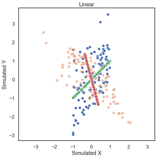
First, let’s generate some simulated data. The k-sample simulations included take on required parameters an independence simulation from the the sims module, number of samples, and number of dimensions with optional paramaters mentioned in the reference section of the docs. Looking at some linearly distributed data first, let’s look at 100 samples of noisey data and generate a 2-dimensional simulation that is rotated by 60 degrees (a 1000 sample of no noise simulated data shows the trend in the data).

# hyppo code used to produce the simulation data
samp1, samp2 = rot_2samp(linear, 100, 1, degree=60, noise=True)
samp1_no_noise, samp2_no_noise = rot_2samp(linear, 1000, 1, degree=60, noise=False)


# stuff to make the plot and make it look nice
fig = plt.figure(figsize=(8,8))
ax = sns.scatterplot(samp1[:, 0], samp1[:, 1])
ax = sns.scatterplot(samp2[:, 0], samp2[:, 1], alpha=0.5)
ax = sns.scatterplot(samp1_no_noise[:, 0], samp1_no_noise[:, 1])
ax = sns.scatterplot(samp2_no_noise[:, 0], samp2_no_noise[:, 1], alpha=0.5)
ax.set_xlabel('Simulated X')
ax.set_ylabel('Simulated Y')
plt.title("Linear")
plt.axis('equal')
plt.show()

The test statistic the p-value is calculated by running the .test method. Some important parameters for the .test method:

• indep_test: This is a required parameter which is a string corresponding to the name of the class for which the non-parametric independence test will be run
• reps: The number of replications to run when running a permutation test
• workers: The number of cores to parallelize over when running a permutation test

The last two parameters are equivalent to and work the same as those in the independence module. Note that when using a permutation test, the lowest p-value is the reciprocal of the number of repetitions. Also, since the p-value is calculated with a random permutation test, there will be a slight variance in p-values with subsequent runs.

# test statistic and p-values can be calculated for MGC, but a little slow ...
stat, pvalue = KSample("Dcorr").test(samp1, samp2)

print("Energy test statistic:", stat)
print("Energy p-value:", pvalue)

Energy test statistic: 0.04436470736551818
Energy p-value: 0.001

# so fewer reps can be used, while giving a less confident p-value ...
stat, pvalue = KSample("Dcorr").test(samp1, samp2, reps=100)

print("Energy test statistic:", stat)
print("Energy p-value:", pvalue)

Energy test statistic: 0.04436470736551818
Energy p-value: 0.01

/Users/sampan501/workspace/hyppo/hyppo/_utils.py:67: RuntimeWarning: The number of replications is low (under 1000), and p-value calculations may be unreliable. Use the p-value result, with caution!
  warnings.warn(msg, RuntimeWarning)

# or the parallelization can be used (-1 uses all cores)
stat, pvalue = KSample("Dcorr").test(samp1, samp2, workers=-1)

print("Energy test statistic:", stat)
print("Energy p-value:", pvalue)

Energy test statistic: 0.04436470736551818
Energy p-value: 0.001

We see that Energy is able to detect linear relationships very easily (p-value is less than the alpha level of 0.05).

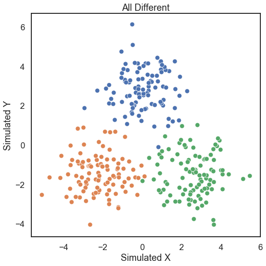
It is easy to use our k-sample tests for 3 samples as well. Let’s look at some random multivariate Gaussian simulations. Case 3 is when all Gaussians are moving away from the origin according to the epsilon parameter.

# hyppo code used to produce the simulation data
samp1, samp2, samp3 = gaussian_3samp(100, case=3, epsilon=5)


# stuff to make the plot and make it look nice
fig = plt.figure(figsize=(8,8))
ax = sns.scatterplot(samp1[:, 0], samp1[:, 1])
ax = sns.scatterplot(samp2[:, 0], samp2[:, 1])
ax = sns.scatterplot(samp3[:, 0], samp3[:, 1])
ax.set_xlabel('Simulated X')
ax.set_ylabel('Simulated Y')
plt.title("All Different")
plt.axis('equal')
plt.show()

stat, pvalue = KSample("Dcorr").test(samp1, samp2, samp3)

print("DISCO test statistic:", stat)
print("DISCO p-value:", pvalue)

DISCO test statistic: 0.8485965561961212
DISCO p-value: 0.001